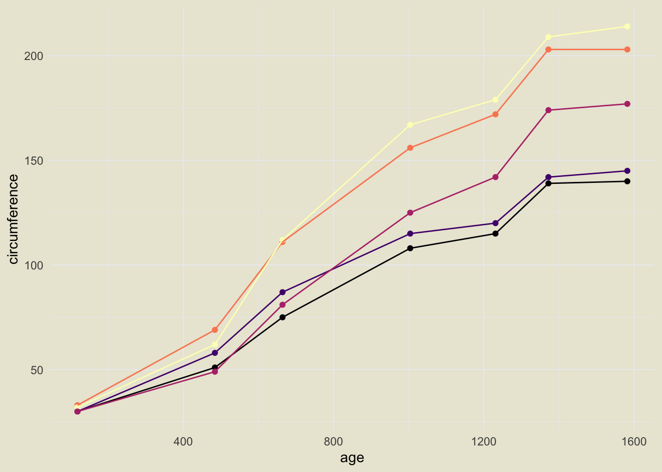
Who knew? Data science is trendy, and I’m looking to get into it. See, look- I’m already DOING data science right here:

library(tidyverse)
library(ggplot2)

oplot <- ggplot(Orange, aes(x = age, 
                   y = circumference, 
                   colour = Tree)) +
  geom_point() +
  geom_line() +
  guides(colour = FALSE) +
  theme_minimal() +
  scale_colour_viridis_d(option = "magma") +
  theme(
    plot.background = element_rect(fill = "#EAE7D6", colour = NA))
oplot

Gotta say- I love these viridis palettes. I think magma is my favorite! Here is a markdown image inserted using ![](magma.jpg)

I also sometimes use knitr for this kind of thing too:

knitr::include_graphics("magma.jpg")

As you can tell from my bio, I like fun colors.

I use lots of colors in my new children’s book too.

Here is a link to my the Saved by the Bell logo in static folder.

Here is the actual image

Here is a link to another one of my posts: here

Oh and you guys? I learned a new thing! Here are some relative links made with blogdown shortcodes:

link to my bio

link to jupyter post

I can’t get it to work with static/ links though.

Let’s read in that Orange data frame:

happy <- readr::read_csv("orange-you-happy.csv")

## Parsed with column specification:
## cols(
##   Tree = col_double(),
##   age = col_double(),
##   circumference = col_double()
## )

dplyr::glimpse(happy)

## Observations: 35
## Variables: 3
## $ Tree          <dbl> 1, 1, 1, 1, 1, 1, 1, 2, 2, 2, 2, 2, 2, 2, 3, 3, 3,…
## $ age           <dbl> 118, 484, 664, 1004, 1231, 1372, 1582, 118, 484, 6…
## $ circumference <dbl> 30, 58, 87, 115, 120, 142, 145, 33, 69, 111, 156, …